The topic discussed in this post is a routine calculation, usually related to FG cut and fill quantities. Occasionally, a client has some fill stockpiled and wants the volume to determine how much additional fill he or she may need.
The following example is intended to show how to derive a volume of a portion of a surface. The overall procedure involved is the same no matter whether you are performing quantity calculations on FG fill, or simply want to see how much dirt you need to store after digging that goldfish pond you always wanted. (It’s just an example, not a desire! If I can’t cornmeal it and fry it, I’m not digging a pond for it).
The steps involved are fairly simple:
- Create the sample surface
- Identify the limits of the volume calculation
- Create a comparison surface
- Create a volume surface
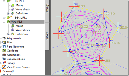
Notice in the following image, the Surface named ‘EG-SURF1’. You should be able to identify the 3 mounds piled together, and the data points that established them.
Identify the limits of the volume calculation
In order to create a comparison surface the limits of the subject (the fill) has to be determined. In this case, the toe of slope is where the piles stop, and natural ground begin. I have created a polyline around the base of the piles, using the toe locations. I will use this as my base for a Feature Line, and for the boundary of the surface as well.
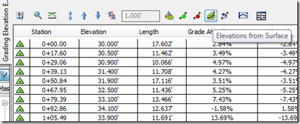
I have created a Feature Line using the Polyline mentioned previously. In the Feature Line Elevation Editor, I have selected the ‘Elevations From Surface’ button, and assigned the Surface elevations directly to the Feature Line. The result is a duplicate of the ‘Base” of the pile using the identical points the sample surface was created with. This method will help limit the inherent abnormalities in the resulting Volume Surface.
Create a comparison surface
In order to make the comparison, I need another surface. I have a feature line, but nothing to assign it to. So I have created an empty Tin Surface. Now I can Right Click the Feature Line, and select ‘Add to Surface as Breakline’.
POOF! A Surface representing the ‘Floor’ of the pile is created. You may notice some stray triangles along the edge(in your practice), and would opt for a Boundary to be added to the definition. In this case, the Boundary is already available. Use the Feature Line for the Boundary. After the surface updates, this is what we get. Nice.
Now the fun begins.
Create a volume surface
Civil 3D was designed to make this routine job easier. The Volume Surface can be created from the Create Surface dialog, and are available as Tin and Grid Surfaces. If you came from LDD, you will soon find out how much easier this is.
After opting to create a new surface, the Create Surface dialog appears as usual. Under Type, I have chosen the Volume Surface that suits my needs best. GRID.
Below you should see the Grid Volume surface I have created, and the settings I have changed. The key features here that I want to focus on are the Grid Spacing, and the Surfaces in the comparison.
This is a small pile, and I have used 1 foot for my spacing. I can afford to go much smaller on the sampling, but there really is no need here. Use some judgment with regard to the spacing. Too small and the memory needed to calculate and store that data goes way up. Too large and the volumes are far too inaccurate.
In order to get the CUT/FILL data identified properly in the CUT/FILL fields, and not backwards, it is useful to think of this as a subtraction problem. Say it to yourself: “I want to subtract the BASE from the COMPARISON”. In most cases this would be like saying, “I want to subtract the EG from the FG”. If you can remember that, your CUT/FILL should be shown properly.
In the Volume Surface properties, select the Statistics Tab. Under Volume, the Cut and Fill volumes are now available. I Love Civil 3D.
Irregularities
Volume Surfaces are not related to the datum of your surface. The data In the Volume Surface is related to the Base Surface. All the elevated data contained therein is relative to 0. This means that the surface elevations start at 0′ along the bottom of the Volume Surface, not at 30′ like the data sampled. This is why the Volume contours are not directly on top of the sampled contours.
Nothing is perfect. In the image above, you can see that not only do the Volume contours not lie on top of the Sampled contours, but the relative shape is slightly different. This is due to the nature of the sampling method, in this case, the 1′ grid is not an exact representation of the sampled surface, however in many cases it is a better model that a Tin Volume.
Later, I will discuss the differences between Grid and Tin volume Surfaces, and how the resulting irregularities occur.
I will also show how to get the resulting surface model nearly identical. Again, that is not necessary in most cases, and is a huge waste of time, and memory. However understanding how this works will help you make better judgments about the type of surface you will use in the future.


